Decay amount, elapsed time, half-life & starting quantity
—
remaining
Enter values and calculate
Decay constant (λ)—
Mean lifetime (τ)—
Half-lives elapsed—
Decay curve (0–5 half-lives)
Common isotope half-lives (tap a row to load it)
Isotope
Half-life
Typical use
N(t) = N₀ × 0.5^(t / T) — decay model assumes a constant half-life.
🔗 Explore connected calculators
A Half Life Calculator is a simple way to calculate how much of a substance remains after a certain amount of time based on its half-life. Instead of manually working through logarithms and exponential equations, you can enter the required values and get the result quickly.
The calculator can be useful for students studying chemistry and physics, teachers preparing examples, researchers performing preliminary calculations, and anyone who wants to understand exponential decay.
At its simplest, half-life means the amount of time required for a quantity to decrease to half of its current value.
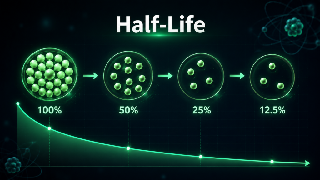
For example, if you begin with 100 grams of a radioactive substance and its half-life is 10 years, 50 grams will remain after 10 years. After another 10 years, 25 grams will remain. After another 10 years, 12.5 grams will remain.
The important thing to remember is that the quantity is repeatedly divided by two. It does not decrease by the same fixed amount during every time interval.
Our calculator uses this exponential decay behavior to determine the remaining quantity, elapsed time, half-life, or initial amount.
Table of Contents
What Is Half-Life?
Half-life is the time required for half of a quantity undergoing radioactive decay to decay.
In nuclear physics, every radioactive nuclide has a characteristic half-life. The process is statistical: it is not possible to predict exactly when an individual unstable nucleus will decay, but the behavior of a large population of nuclei can be modeled very accurately.
OpenStax describes radioactive decay as a first-order process and defines the half-life as the time required for half of the atoms in a sample to decay.
The concept can be demonstrated with a simple example.
Imagine that a substance has a half-life of 5 years and starts with 100 units:
Time
Half-lives elapsed
Amount remaining
0 years
0
100
5 years
1
50
10 years
2
25
15 years
3
12.5
20 years
4
6.25
25 years
5
3.125
Notice that the amount removed during each interval gets smaller.
During the first five years, 50 units disappear.
During the next five years, only 25 units disappear.
During the following five years, 12.5 units disappear.
This is the characteristic behavior of exponential decay.
How Does a Half Life Calculator Work?
The calculator is based on the standard radioactive decay relationship:
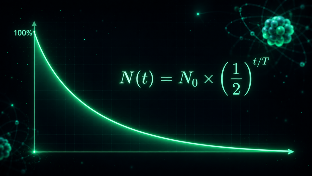
N(t) = N₀ × (1/2)^(t/T)
Where:
N(t) = quantity remaining after time t
N₀ = initial quantity
t = elapsed time
T = half-life
The term t/T represents the number of half-lives that have passed.
For example, if a substance has a half-life of 5 years and 20 years have passed:
t/T = 20/5 = 4
Four half-lives have elapsed.
The remaining fraction is therefore:
(1/2)^4 = 1/16
That means 6.25% of the original amount remains.
A Half Life Calculator performs this calculation automatically. This becomes particularly useful when the elapsed time is not an exact multiple of the half-life.
For example, calculating the remaining amount after 7.3 years when the half-life is 5.27 years involves a fractional exponent. A calculator avoids the need to manually evaluate that expression.
How to Use the Half Life Calculator
Using the calculator is straightforward. The exact fields depend on which calculation mode you select.
Step 1: Select the calculation you want
The calculator provides different calculation modes, including:
Remaining Amount
Elapsed Time
Half-Life
Initial Amount
If you want to know how much remains after a certain period, select Remaining Amount.
If you know the starting and ending quantities and want to find how long the process took, select Elapsed Time.
Step 2: Select an isotope preset
If the calculator provides an isotope preset, you can select a commonly known isotope rather than entering its half-life manually.
For example, the calculator shown above includes Cobalt-60 (5.27 yr).
Cobalt-60 has a half-life of approximately 5.27 years according to OpenStax, while NIST reports a value of approximately 5.26 years on its Cobalt-60 reference page. Small differences in displayed values can occur because of rounding and the precision used by different references.
For scientific or regulatory work, always use the half-life value specified by the appropriate authoritative reference.
Step 3: Enter the initial quantity
Enter the starting quantity in the Initial Quantity (N₀) field.
The value could represent:
grams
kilograms
moles
number of atoms
activity
another quantity represented by the decay model
The calculator does not need to know the physical unit of the quantity itself for the mathematical decay calculation. What matters is that the starting and remaining quantities use the same unit.
For example:
Initial quantity = 100 grams
The result will be expressed in grams.
If you enter:
Initial quantity = 500 atoms
the calculated result represents the number of atoms remaining according to the mathematical model.
Step 4: Enter the half-life
Enter the half-life and select the appropriate time unit.
For example:
Half-life = 5.27 years
or:
Half-life = 120 minutes
The important thing is to use compatible units for half-life and elapsed time.
Step 5: Enter the elapsed time
Enter the amount of time that has passed.
For example:
Elapsed time = 10 years
If the half-life is entered in years, the calculation is straightforward.
If the half-life and elapsed time use different units, they need to be converted to compatible units before applying the equation unless the calculator automatically handles the conversion.
Step 6: Click Calculate
After entering the values, click Calculate.
The calculator provides the requested result and may also display supporting information such as:
Remaining amount
Percentage remaining
Decay constant
Mean lifetime
Number of half-lives elapsed
Decay curve
These additional values can help you understand not just the answer, but also what is happening mathematically.
Half-Life Formula Explained
The most commonly used half-life formula is:
N(t) = N₀ × (1/2)^(t/T)
This equation is especially convenient because it directly uses the half-life.
There is another equivalent form based on the decay constant:
N(t) = N₀e^(-λt)
Here, λ, pronounced lambda, is the decay constant.
The relationship between half-life and decay constant is:
λ = ln(2) / T
or approximately:
λ = 0.693 / T
OpenStax provides this relationship and explains that radioactive decay follows first-order kinetics.
Both equations describe the same exponential decay process.
The half-life version is often easier for basic calculations because most radioactive isotope data is given in terms of half-life.
What Is the Decay Constant?
The decay constant, represented by λ, describes the probability rate associated with radioactive decay.
A larger decay constant corresponds to a faster decay process.
A smaller decay constant corresponds to a slower decay process.
Because:
λ = ln(2) / T
an isotope with a short half-life has a relatively large decay constant, while an isotope with a long half-life has a relatively small decay constant.
For example, if a substance has a half-life of 10 minutes, its decay constant will be much larger than that of a substance with a half-life of 10 years.
Your calculator may show the decay constant alongside the main result. This is useful when studying the connection between exponential decay and half-life.
What Is Mean Lifetime?
Mean lifetime is another quantity associated with exponential decay.
It is represented by:
τ = 1/λ
Because:
λ = ln(2)/T
the mean lifetime can also be written as:
τ = T/ln(2)
or approximately:
τ = 1.443T
Mean lifetime should not be confused with half-life.
Half-life tells you how long it takes for half the original population to decay.
Mean lifetime is a statistical average associated with the exponential decay distribution.
Example 1: Calculate Remaining Amount
Suppose you start with 100 grams of a radioactive substance.
Its half-life is 10 years.
How much remains after 30 years?
Given:
Initial quantity = 100 g
Half-life = 10 years
Elapsed time = 30 years
First calculate the number of half-lives:
30 / 10 = 3
So three half-lives have passed.
Now apply the equation:
N = 100 × (1/2)^3
N = 100 × 1/8
N = 12.5 g
Answer:
12.5 grams remain after 30 years.
This is one of the easiest types of problems because the elapsed time is an exact multiple of the half-life.
Example 2: Calculate Remaining Amount After a Fractional Half-Life
Now suppose the initial amount is 100 grams, the half-life is 10 years, and the elapsed time is 15 years.
The number of half-lives is:
15 / 10 = 1.5
Therefore:
N = 100 × (1/2)^1.5
The result is approximately:
35.36 grams
So approximately 35.36% of the original quantity remains.
This is a good example of when a radioactive decay calculator becomes more convenient than manually calculating the exponential expression.
Example 3: Cobalt-60
Cobalt-60 is a commonly used example when studying radioactive decay.
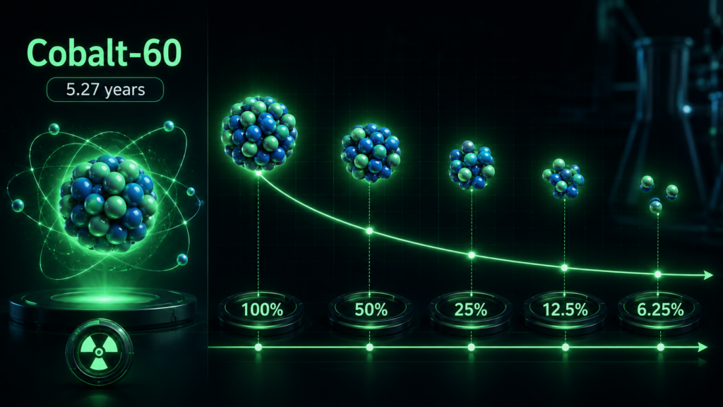
OpenStax lists its half-life as approximately 5.27 years. NIST also documents Cobalt-60 and describes its use in radiation measurement and calibration applications.
Suppose a sample starts with 100 units of Cobalt-60.
After one half-life:
100 → 50
After two half-lives:
50 → 25
After three half-lives:
25 → 12.5
Therefore:
Time
Approximate amount remaining
0 years
100
5.27 years
50
10.54 years
25
15.81 years
12.5
21.08 years
6.25
26.35 years
3.125
These values follow directly from the half-life relationship. OpenStax provides the same sequence for Cobalt-60.
Example 4: Find Elapsed Time
A sample initially contains 800 grams.
After some time, only 100 grams remain.
The half-life is 5 years.
How much time has passed?
Look at the sequence:
800 → 400 → 200 → 100
Three half-lives have elapsed.
Therefore:
Elapsed time = 3 × 5
Elapsed time = 15 years
So approximately 15 years have passed.
For values that do not correspond to an exact number of half-lives, a logarithmic calculation is required.
Example 5: Find the Half-Life
Suppose a sample initially contains 400 grams.
After 18 years, only 100 grams remain.
The quantity changed as follows:
400 → 200 → 100
That represents two half-lives.
Therefore:
Half-life = 18 / 2
Half-life = 9 years
So the estimated half-life is 9 years.
For more complicated values, a half-life equation calculator can solve the rearranged equation automatically.
Example 6: Find the Initial Amount
Suppose you know that a substance has a half-life of 4 years.
After 12 years, the remaining quantity is 25 grams.
How much was present originally?
Twelve years represents:
12 / 4 = 3 half-lives
After three half-lives, only 1/8 of the original amount remains.
Therefore:
Initial amount = 25 × 8
Initial amount = 200 grams
So the starting amount was 200 grams.
Why Does the Calculator Show 0.00%?
A common question when using a Half Life Calculator is why the result sometimes displays a very small percentage or even appears as zero.
The reason is that exponential decay can make the remaining quantity extremely small after many half-lives.
For example:
Half-lives
Percentage remaining
1
50%
2
25%
3
12.5%
4
6.25%
5
3.125%
10
0.0977%
20
0.000095%
After enough half-lives, the actual calculated value can be so small that the calculator rounds it to 0.00% for display.
This does not necessarily mean that the mathematical result is exactly zero.
The exponential model approaches zero asymptotically.
How Many Half-Lives Does It Take to Reach Zero?
Mathematically, exponential decay does not reach exactly zero after a finite number of half-lives.
Instead, it continually gets smaller.
After five half-lives:
1/32 = 3.125%
After ten:
1/1024 ≈ 0.0977%
After twenty:
1/1,048,576 ≈ 0.000095%
This explains why a calculator may show an extremely small amount after a long period.
In practical situations, however, a quantity can become negligible for a particular purpose long before the mathematical value reaches zero.
Understanding the Decay Curve
The decay graph displayed by the calculator provides a visual representation of exponential decay.
At 0T, the quantity is 100%.
At 1T, 50% remains.
At 2T, 25% remains.
At 3T, 12.5% remains.
At 4T, 6.25% remains.
At 5T, 3.125% remains.
The curve drops rapidly at the beginning and becomes progressively flatter.
This shape is fundamentally different from a straight-line graph.
In linear decay, the same absolute quantity is removed during each interval.
In exponential decay, the same fraction is removed during each half-life.
That distinction is one of the most important concepts to understand when working with radioactive decay.
Half-Life vs. Linear Decay
Consider two hypothetical processes.
Linear decrease
Start with 100 units and lose 10 units every year:
100 → 90 → 80 → 70 → 60
The same amount disappears every year.
Exponential decay
Start with 100 units and lose half every period:
100 → 50 → 25 → 12.5 → 6.25
The amount lost gets progressively smaller.
Radioactive decay follows the second pattern.
This is why simply subtracting a fixed percentage or quantity from the original value can produce an incorrect result.
Why Time Units Matter
Unit consistency is one of the most common sources of mistakes.
Suppose an isotope has a half-life of 5 years, but you enter an elapsed time of 120 hours.
The values are not directly compatible.
You need to express both values in the same time unit.
For example:
5 years × 365 days × 24 hours = 43,800 hours
Now you can compare:
Half-life = 43,800 hours
Elapsed time = 120 hours
The same principle applies to seconds, minutes, hours, days, and years.
Always check the units before calculating.
Common Mistakes When Using a Half Life Calculator
1. Thinking one half-life means complete decay
One half-life means 50% remains, not zero.
2. Subtracting half of the original amount every time
The amount that decays during the next half-life is based on what remains.
For example:
100 → 50 → 25 → 12.5
The second reduction is 25, not another 50.
3. Mixing time units
Make sure the half-life and elapsed time are compatible.
4. Entering the wrong initial quantity
The starting value should be entered as the quantity present at time zero.
5. Confusing half-life with decay constant
They are related but are not the same measurement.
6. Assuming every radioactive isotope has the same half-life
Each radioactive nuclide has its own characteristic half-life.
OpenStax provides reference tables showing how dramatically half-lives can vary among isotopes.
Applications of Half-Life Calculations
Half-life is not just a classroom concept. It has important applications in science, engineering, medicine, and environmental studies.
Radioactive dating
Radiometric dating uses radioactive decay and known half-lives to estimate the age of materials.
Carbon-14, for example, is used in radiocarbon dating of suitable carbon-containing materials. OpenStax discusses radiometric dating and the use of radioactive isotopes for determining the age of archaeological and geological materials.
Nuclear medicine
Radioactive isotopes are used in diagnostic imaging and medical treatment.
Understanding how activity changes with time is important when selecting and using radioactive tracers and therapeutic isotopes.
Nuclear engineering
Half-life calculations are relevant to radioactive materials, nuclear facilities, radiation monitoring, and radioactive waste management.
Environmental science
Scientists can use radioactive decay models to study the behavior and persistence of radioactive contaminants.
Education
Half-life provides a practical example of:
exponential functions
logarithms
probability
nuclear physics
first-order kinetics
mathematical modeling
Half-Life and Radioactive Activity
It is important to distinguish the amount of radioactive material from its activity.
Activity refers to the rate of radioactive decays, typically measured in becquerels (Bq), where one becquerel corresponds to one decay per second.
For a radioactive sample:
Activity = λN
As the number of radioactive nuclei decreases, the activity also decreases under the standard decay model.
OpenStax explains the relationship between decay constant, number of nuclei, and radioactive activity.
This is why radioactive sources become less active over time.
Half Life Calculator for Students
Students often encounter half-life questions in chemistry, physics, and nuclear science.
The best approach is to understand the relationship before relying on the calculator.
When solving a problem manually, identify:
The initial quantity.
The half-life.
The elapsed time.
The quantity you need to find.
Whether the time units are consistent.
Then select the appropriate calculation mode in the calculator.
Using the tool alongside manual calculations can also be useful for checking homework and verifying whether your final answer is reasonable.
Half Life Calculator for Cobalt-60
Cobalt-60 is one of the isotope presets that may be useful when demonstrating the calculator.
A commonly used rounded half-life for Cobalt-60 is 5.27 years. NIST documents a value of approximately 5.26 years, while OpenStax uses 5.27 years.
If the calculator uses 5.27 years and you enter an elapsed time of 15.81 years:
15.81 / 5.27 = 3
Three half-lives have passed.
Therefore:
Remaining fraction = (1/2)^3
Remaining fraction = 0.125
So:
12.5% remains
If the initial quantity is 100 units:
Remaining amount = 12.5 units
This is a simple example of how the isotope preset and calculator can work together.
Frequently Asked Questions
What is a Half Life Calculator?
A Half Life Calculator is an online tool that uses the mathematical relationship between half-life, elapsed time, initial quantity, and remaining quantity to calculate radioactive or exponential decay. Depending on the calculator's available modes, it can also solve for elapsed time, half-life, or initial amount.
What is the basic half-life equation?
The basic equation is: N(t) = N₀ × (1/2)^(t/T) N₀ is the initial quantity, N(t) is the remaining quantity, t is elapsed time, and T is the half-life.
How do I calculate the amount remaining after a half-life?
After exactly one half-life, 50% remains. After two half-lives, 25% remains. After three half-lives, 12.5% remains. For fractional half-lives, use the full exponential equation.
Does half-life mean half the material disappears?
Yes, after one half-life, half of the original radioactive population has decayed. However, another half of the remaining population decays during the next half-life. Therefore, the amount does not reach zero after two or three half-lives.
What remains after five half-lives?
After five half-lives: (1/2)^5 = 1/32 Therefore, 3.125% remains.
What remains after ten half-lives?
After ten half-lives: (1/2)^10 = 1/1024 Approximately 0.0977% remains.
Can the calculator find elapsed time?
Yes. If the initial quantity, remaining quantity, and half-life are known, elapsed time can be calculated using a rearranged logarithmic form of the decay equation.
What is the difference between half-life and decay constant?
Half-life is the time required for half of a radioactive population to decay. The decay constant represents the rate parameter of the exponential decay process. They are related by: λ = ln(2)/T
Half Life Calculator: Quick Reference
Calculation
Required information
Result
Remaining Amount
Initial amount, half-life, elapsed time
Amount remaining
Elapsed Time
Initial amount, remaining amount, half-life
Time elapsed
Half-Life
Initial amount, remaining amount, elapsed time
Half-life
Initial Amount
Remaining amount, half-life, elapsed time
Starting amount
The calculator can therefore be used in both forward and reverse calculations rather than simply finding the amount remaining.
Reference Links
For educational and scientific reference, the following sources are useful:
This Half Life Calculator and the information provided on this page are intended for educational and general informational purposes only.
The calculations assume an exponential decay model with a constant half-life. Actual scientific, medical, environmental, or nuclear applications may require additional factors, validated measurements, isotope-specific data, calibration information, and professional analysis.
Do not use this calculator as a substitute for professional radiation-safety advice, medical advice, laboratory measurements, regulatory guidance, or certified nuclear data.
When performing calculations for professional or safety-critical applications, verify the isotope half-life and other relevant parameters using an authoritative scientific or regulatory source.
Conclusion
A Half Life Calculator provides a quick way to understand and calculate exponential decay without manually working through every logarithmic or exponential calculation.
The central concept is simple: after each half-life, half of the remaining quantity is left.
The standard relationship is:
N(t) = N₀ × (1/2)^(t/T)
From this equation, you can calculate the remaining amount, elapsed time, half-life, or initial quantity when the necessary values are known.
For simple problems, you can often calculate the answer by repeatedly dividing the starting quantity by two. For more complicated calculations involving fractional half-lives, large numbers, or very long periods, an online calculator makes the process considerably easier.
Whether you are studying radioactive decay, working through a chemistry assignment, learning nuclear physics, or simply exploring exponential decay, the calculator can help you understand both the numerical result and the behavior behind it.
The most important thing is to use the correct half-life, maintain consistent time units, and understand what the calculated value represents.
Once those basics are clear, even complex-looking half-life problems become much easier to solve.
Related Posts
About Smith Ghule
Hi, I’m Smith Ghule — a passionate cricket enthusiast and technology professional from Pune, Maharashtra. I have been working in the IT industry since 2015, gaining experience across various domains in technology and operations. Alongside my professional journey, I closely follow cricket and enjoy staying updated with the latest developments in both the sports and tech worlds. My interests lie in combining analytical thinking, innovation, and continuous learning to grow personally and professionally.